If you want to try out our example implementation of Interactive Timing Analysis, you can use this guide:
Steps for setup:
- Download the KIELER SCCharts editor with Interactive Timing Analysis here. Choose the release, i.e. the
KIELER SCCharts Product v. 0.11.0 (2014-02-28, based on Eclipse 4.3 Kepler) in the right version for your platform. - Get the experimental KTA timing analysis tool here. You can download the ZIP folder.
- Make sure ocaml and "make" are installed on your system, so that you can compile the KTA timing analysis tool.
- Extract the zip folder you downloaded in Step 2 and compile the KTA timing analysis tool running make in the kta-master folder.
- Install the gcc MIPS compiler (mcb32tools, mipsel-mcb32-elf-gcc), which is used by the KTA timing analysis tool.
- Start up KIELER, go to Preferences -> Interactive Timing Analysis and enter the absolute paths in your system to the folder that
contains the KTA tool binary or the gcc MIPS compiler, respectively (click image to enlarge):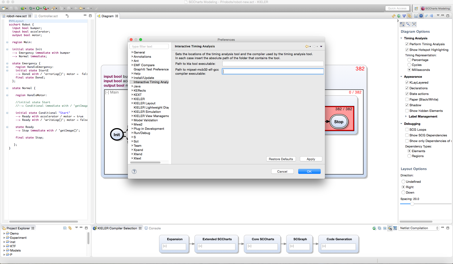
How to use the Interactive Timing Analysis:
You can use this selection of example models to get you started: TestFilesTiming.
- Create a Project in your Project Explorer (right click -> New -> Project).
- Copy the files and folders contained in the TimingTestFiles folder into the Project.
- Make sure the folders that contain the .sct and .asu file of the models and the tpp.h file are on one level, like in the TimingTestFiles folder.
- Open any of the .sct files in the editor (right click the file). The Diagram view should open automatically and show you an image of the model. If that does not work, open that view by choosing Window -> Show View -> Other -> KIELER Lightweight Diagrams -> Diagram
- Choose your desired Timing Analysis Options in the Diagram Options bar (click image to enlarge):
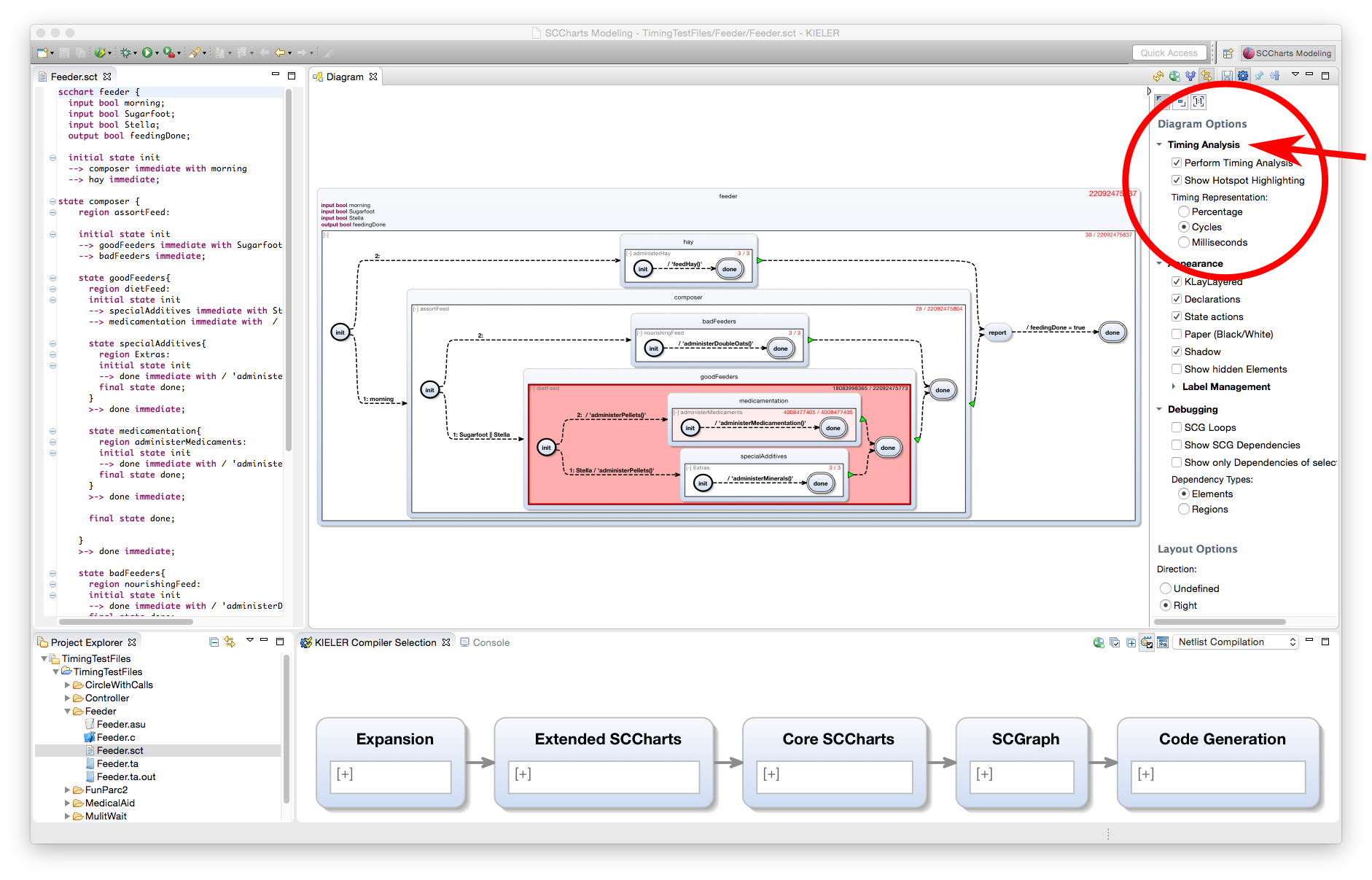
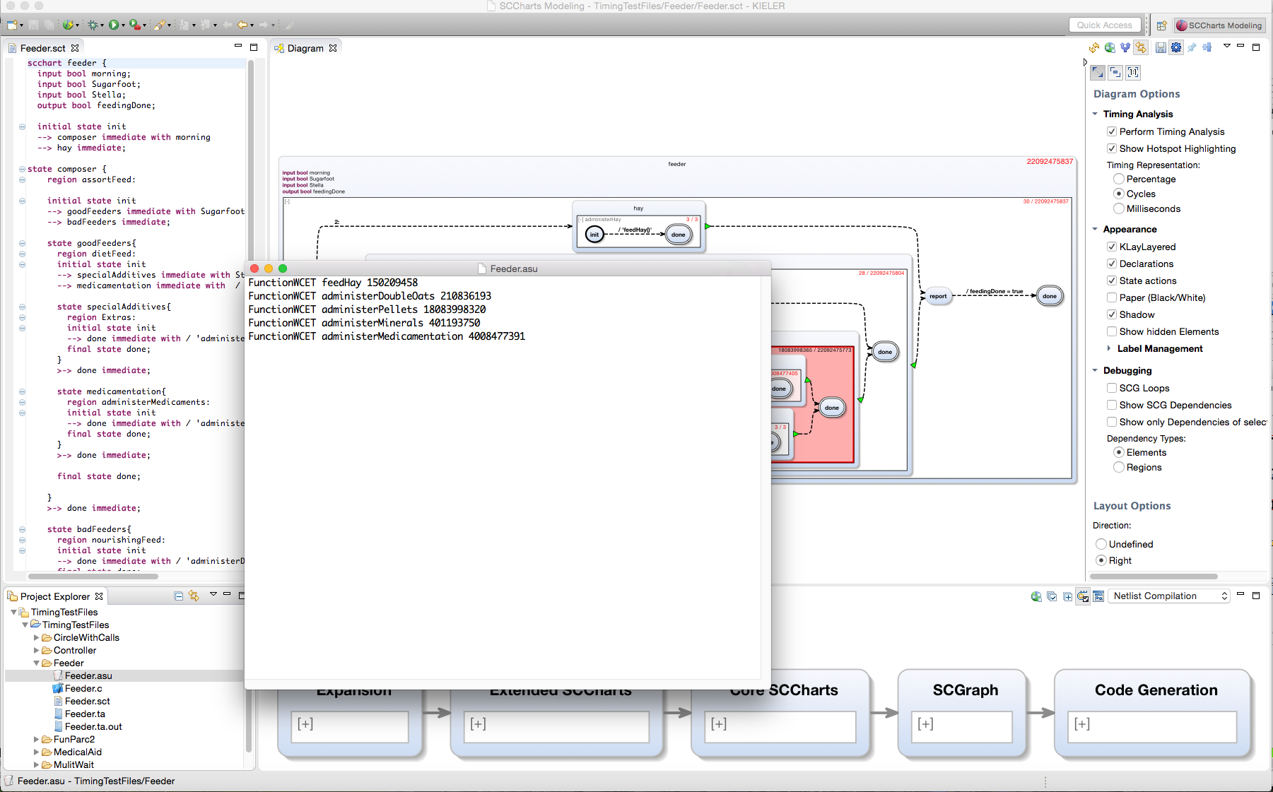
You can switch between percentage, cycles and milliseconds for the timing value display. You can of course also try out the other Diagram and Layout Options in the bar. - As a first step you can play around with the timing assumptions on function calls you find in the .asu files for the models (note that FunParc2 has no function calls, so choose something else):
- You can see how the values and the Hotspot Highlighting change when you update the view by clicking on the button with this symbol:

- Try to create and edit your own models (right click the project -> new -> Folder, then right click the folder -> new -> file, give the file a name that ends with .sct). You can edit your file in the textual editor now. Please note that you have to add an assumption file with the same name as the model file, but the ending .asu that contains timing assumptions for any function call you use in your model. Your diagram view is updated with every save. Also, your timing values are recomputed and displayed.
For a quick start guide on SCCharts and how to model them see also this page.
If you encounter problems trying out the Interactive Timing Analysis, please contact Insa Fuhrmann: ima@informatik.uni-kiel.de
Overview
Content Tools