Page History
| Panel | ||||||
|---|---|---|---|---|---|---|
|
| |||||
Responsible: Key Publications:
Further Publications:
Related Theses:
|
KLay Layered is a layer-based layout algorithm mainly intended for diagrams with an inherent data flow direction. This page describes the architecture and its general architecture, while child pages discuss the different phases of the KLay Layered algorithm, as well as some notable features that may require further explanation, its intermediate processors, and other specialized topics.
Contents
| Table of Contents | ||
|---|---|---|
|
| Excerpt Include | ||||
|---|---|---|---|---|
|
Architecture
To get an idea of how KLay Layered is structured, take a look at the diagram below. The algorithm basically consists of just three four components: layout phases, intermediate processors, a connected components processor, and an interface to the outside world. Let's briefly look at what each component does before delving into the gritty details.
...
The backbone of KLay Layered are its five layout phases, of which each is performing a specific part of the work necessary to layout a graph. The Three of the five phases (layer assignment, crossing minimization, and node placement) go back to a paper by someone whose name I'm currently too lazy to look upSugiyama et al. They are widely used as the basis for layout algorithms, and can be found in loads of papers on the topic. A detailed description of what each layout phase does can be found below on this page.
Intermediate processors are less prevalent. In fact, it's they are one of our contributions to the world of layout algorithms. The idea here is that we want KLay Layered to be as generic as possible, supporting different kinds of diagrams, laid out in different kinds of ways . (as long as the layout is based on layers). Thus, we are well motivated to keep the layout phases as simple as possible. To adapt the algorithm to different needs, we then introduced small processors between the main layout phases . (the space between two layout phases is called a a slot) One . One processor can appear in different slots, and one slot can be occupied by more than one processor. Processors usually modify the graph to be laid out in ways that allow the main phases to solve problems they wouldn't solve otherwise. That's an abstract enough explanation for it to mean anything and nothing at once, so let's take a look at a short example.
As will be seen below, the The task of phase 2 is to produce a layering of the graph. The result is that each node is assigned to a layer in a way that edges always point to a node in a higher layer. However, later phases may require the layering to be proper. (a layering is said to be proper if two nodes being connected by an edge are assigned to neighboring layers). Instead of modifying the layerer to check if a proper layering is needed, we introduced an intermediate processors processor that turns a layering into a proper layering. Phases that need a proper layering can then just indicate that they want that processor to be placed in one of the slots.
For graphs that are not connected it is possible to execute the algorithm, i.e. the five phases with intermediate processors, separately on each connected component. The connected components processor splits an unconnected graph into multiple connected graphs and rearranges them after the layout of each component has been computed. This helps to present the components more compactly and neatly.
The interface to the outside world finally allows us to plug our algorithm into the programs wanting to use it. While not strictly part of the actual algorithm, that interface allows us to lay out graphs people throw at us regardless of the data structures used to represent those graphs. Internally, KLay Layered uses a data structure called LGraph to represent graphs. (an LGraph can be thought of as a lightweight version of KGraph, with the concept of layers added) All a potential user has to do is write an import and export module to make his graph structure work with KLay Layered. Currently, the there's only two module available is the KGraphImporterfor importing KGraphs, which makes make KLay Layered work with KIML: KGraphImporter, which imports a single hierarchy level, and CompoundKGraphImporter, which imports and flattens the whole hierarchy to enable compound graph layout.
More details on the classes relevant to this architecture can be found below.
Dummy Nodes
Before getting down to it, one other thing is worthy of our attention: dummy nodes. Dummy nodes are nodes inserted into the graph during the layout process. They were not in the original graph that is to be laid out, and are removed prior to the layout being applied to the original graph structure. So why then do we need them?
...
See the graph below for an example. The orange nodes were layered, but the layering was by no means a proper layering. Thus, gray dummy nodes were added.
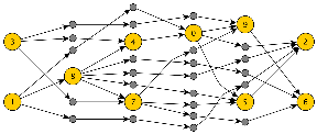
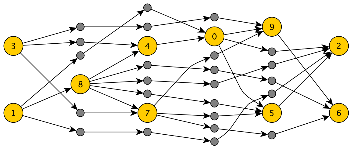
In KLay Layered, we make extensive use of dummy nodes to reduce complex and very specific problems such that we can solve them using our general phases. One example is how we have implemented support for ports our implementation of port support on the northern or southern side of a node.
Phases
This section describes the algorithm's five main phases and the available implementations. You can find a list and descriptions of the intermediate processors below.
Phase 1: Cycle Removal
The first phase makes sure that the graph doesn't contain any cycles. In some papers, this phase is an implicated part of the layering. This is due to the supporting function cycle removal has for layering: without cycles, we can find a topological ordering of the graph's nodes, which greatly simplifies layering.
An important part to note is that cycles may not be broken by removing one of their edges. If we did that, the edge would not be routed later, not to speak of other complications that would ensue. Instead, cycles must be broken by reversing one of their edges. Since the problem of finding the minimal set of edges to reverse to make a graph cycle-free is NP-hard, (or NP-complete? I don't remember from the top of my head) cycle removers will implement some heuristic to do their work.
The reversed edges have to be restored at some point. There's a processor for that, called ReversedEdgeRestorer. All implementations of phase one must include a dependency on that processor, to be included after phase 5.
Precondition
- No node is assigned to a layer yet.
Postcondition
- The graph is now cycle-free. Still, no node is assigned to a layer yet.
Remarks
- All implementations of phase one must include a dependency on the ReversedEdgeRestorer, to be included after phase 5.
Current Implementations
- GreedyCycleBreaker. Uses a greedy approach to cycle-breaking.
Phase 2: Layering
The second phase assigns nodes to layers. (also called ranks in some papers) Nodes in the same layer are assigned the same x coordinate. (give or take) The problem to solve here is to assign each node x a layer i such that each successor of x is in a layer j>i. The only exception are self-loops, that may or may not be supported by later phases.
It must be differentiated between a layering and a proper layering. In a layering, the above condition holds. (well, and self-loops are allowed) In a proper layering, each successor of x is required to be assigned to layer i+1. This is possible only for the simplest cases, but may be required by later phases. In that case, later phases use the LongEdgeSplitter processor to turn a layering into a proper layering by inserting dummy nodes as necessary.
Note that nodes can have a property associated with them that constraints the layers they can be placed in.
Precondition
- The graph is cycle-free.
- The nodes have not been layered yet.
Postcondition
- The graph has a layering.
Remarks
- Implementations should usually include a dependency on the LayerConstraintHandler, unless they already adhere to layer constraints themselves.
Current Implementations
- LongestPathLayerer. Layers nodes according to the longest paths between them. Very simple, but doesn't usually give the best results.
- NetworkSimplexLayerer. A way more sophisticated algorithm whose results are usually very good.
Phase 3: Crossing Reduction
The objective of phase 3 is to determine how the nodes in each layer should be ordered. The order determines the number of edge crossings, and thus is a critical step towards readable diagrams. Unfortunately, the problem is NP-hard even for only two layers. Did I just hear you saying "heuristic"? The usual approach is to sweep through the pairs of layers from left to right and back, along the way applying some heuristic to minimize crossings between each pair of layers. The two most prominent and well-studied kinds of heuristics used here are the barycenter method and the median method. We have currently implemented the former.
Our crossing reduction implementations may or may not support the concepts of node successor constraints and layout groups. The former allows a node x to specify a node y!=x that may only appear after x. Layout groups are groups of nodes. Nodes belonging to different layout groups are not to be interleaved.
Precondition
- The graph has a proper layering. (except for self-loops)
- An implementation may allow in-layer connections.
- Usually, all Nodes are required to have at least fixed port sides.
Postcondition
- The order of nodes in each layer is fixed.
- All nodes have a fixed port order.
Remarks
- If fixed port sides are required, the PortPositionProcessor may be of use.
- Support for in-layer connections may be required to be able to handle certain problems. (odd port sides, for instance)
Current Implementations
- LayerSweepCrossingMinimizer. Does several sweeps across the layers, minimizing the crossings between each pair of layers using a barycenter heuristic. Supports node successor constraints and layout groups. Node successor constraints require one node to appear before another node. Layout groups specify sets of nodes whose nodes must not be interleaved.
Phase 4: Node Placement
So far, the coordinates of the nodes have not been touched. That's about to change in phase 4, which determines the y coordinate. While phase 3 has an impact on the number of edge crossings, phase 4 has an influence on the number of edge bends. Usually, some kind of heuristic is employed to yield a good y coordinate.
Our node placers may or may not support node margins. Node margins define the space occupied by ports, labels and such. The idea is to keep that space free from edges and other nodes.
Precondition
- The graph has a proper layering. (except for self-loops)
- Node orders are fixed.
- Port positions are fixed.
- An implementation may allow in-layer connections.
- An implementation may require node margins to be set.
Postcondition
- Each node is assigned a y coordinate such that no two nodes overlap.
- The height of each layer is set.
- The height of the graph is set to the maximal layer height.
Remarks
- Support for in-layer connections may be required to be able to handle certain problems. (odd port sides, for instance)
- If node margins are supported, the NodeMarginCalculator can compute them.
- Port positions can be fixed by using the PortPositionProcessor.
Current Implementations
- LinearSegmentsNodePlacer. Builds linear segments of nodes that should have the same y coordinate and tries to respect those linear segments. Linear segments are placed according to a barycenter heuristic.
Phase 5: Edge Routing
In the last phase, it's time to determine x coordinates for all nodes and route the edges. The routing may support very different kinds of features, such as support for odd port sides, (input ports that are on the node's right side) orthogonal edges, spline edges etc. Often times, the set of features supported by an edge router largely determines the intermediate processors used during the layout process.
Precondition
- The graph has a proper layering. (except for self-loops)
- Nodes are assigned y coordinates.
- Layer heights are correctly set.
- An implementation may allow in-layer connections.
Postcondition
- Nodes are assigned x coordinates.
- Layer widths are set.
- The graph's width is set.
- The bend points of all edges are set.
Remarks
None.
Current Implementations
...
Class Design
The class design of KLay Layered is probably best explained through the use of the following diagram, which you will now have to enlarge and study (don't worry, we'll explain the different parts in a minute):
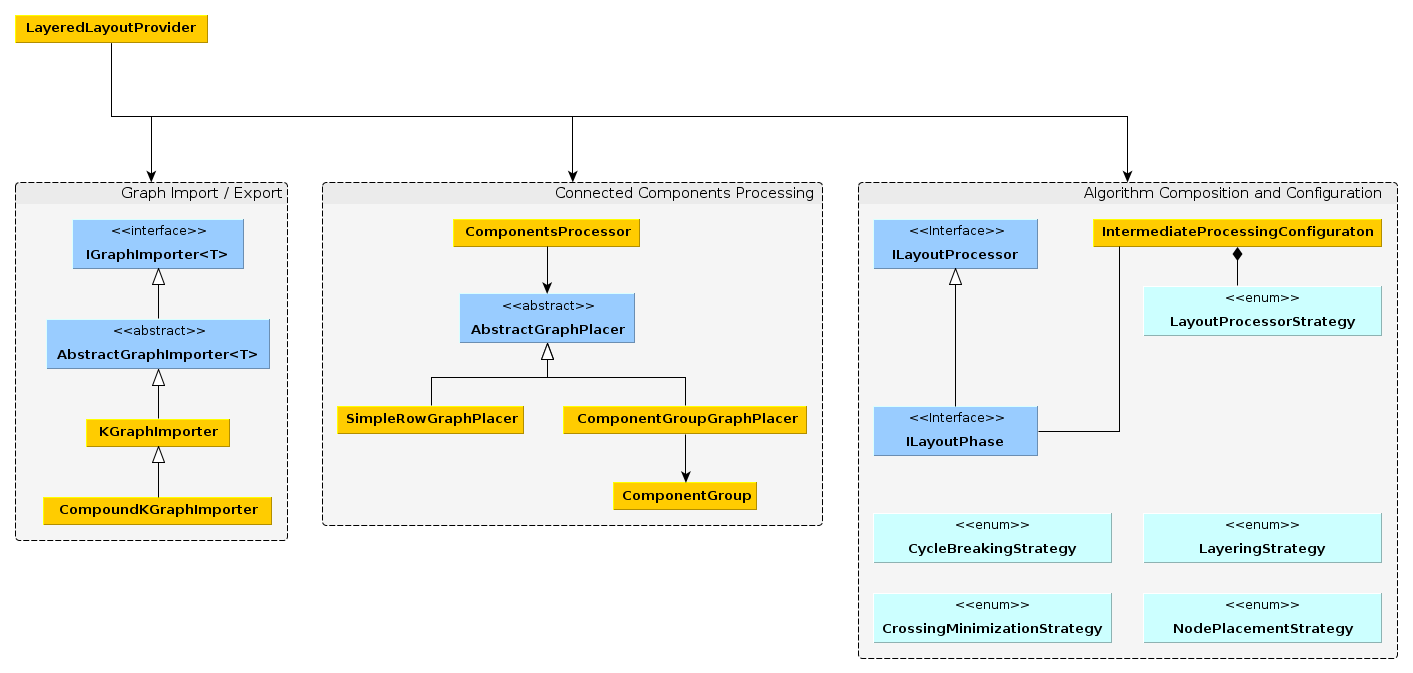
Lets work our way through the diagram.
Graph Import and Export
Since KLay Layered's internal format is the LGraph, we need a way to import KGraphs (maybe also other external formats) into the LGraph format, and a way to apply the computed layout information back to the original graph. This is what IGraphImporter implementations are for. The AbstractGraphImporter predefines methods for handling common import situations, such as generating dummy nodes for hierarchical ports. The KGraphImporter knows how to import and export a single level of hierarchy, while the CompoundKGraphImporter knows how to import the whole hierarchy at once.
Connected Components Processing
Each connected component of a graph can be laid out separately and afterwards placed in a way as to minimize the area taken up by the drawing. This results in much more pleasing and space-efficient layouts than if we were to only consider a graph as a whole. Splitting and rejoining the graph is implemented in the ComponentsProcessor. Splitting is always the same, so the processor just does that itself. Joining connected components, however, can be done in different ways, implemented by different subclasses of AbstractGraphPlacer (which provides commonly used methods to move connected components around). The CompoundGroupGraphPlacer uses a sophisticated algorithm and uses ComponentGroup instances as the data structure to operate on.
Algorithm Composition and Configuration
KLay Layered can flexibly adapt itself to different layout requirements. To that end, the algorithm itself is basically just a list of modules (ILayoutProcessor) that the input graph is passed through. However, the algorithm is still based around the concept of five different layout phases, which implement the ILayoutPhase interface. The algorithm configuration happens like this:
- The input graph is annotated with information as to which concrete implementations of the different layout phases to use. Each phase (except for the last one) has a corresponding strategy enumeration describing the different choices. (Strategy pattern, anyone?) The layout phases are instantiated and form the basic structure of the algorithm.
- Each phase implementation may require a list of ILayoutProcessors to be executed in the different intermediate processing phases. These requirements are described using IntermediateProcessingConfigurations. The requirements of each phase are collected and instantiated.
- From the phase and layout processor instances, the final list of modules is compiled that makes up the currently required incarnation of the algorithm.
Putting It All Together
The central class is the LayeredLayoutProvider. It does the following:
- Using one of the IGraphImporter implementations, it imports the KGraph to be laid out into KLay Layered's LGraph format. Which implementation is used depends on whether the algorithm has to compute a layout for all hierarchy levels at once (compound layout) or not.
- Since the algorithm's configuration depends on the graph to be laid out, the LayeredLayoutProvider now has to decide which ILayoutPhase implementations to use for each of the five layout phases (this is specified with the different phase strategy enumerations). Once that is decided, each ILayoutPhase is queried for an IntermediateProcessingConfiguration, which describes – using the LayoutProcessorStrategy – the ILayoutProcessors it needs in each of the intermediate processing slots. The outcome of this step is a list of ILayoutProcessor instances that constitute the concrete layout algorithm.
- Next, the imported graph is split into its connected components using the ComponentsProcessor. The processor does the work of splitting the graph into its connected components.
- The main step: executing the algorithm (the list of ILayoutProcessor instances, as you will certainly remember) on each connected component.
- With a layout computed for each connected component, the ComponentsProcessor is invoked again to join them together. The processor can use one of two implementations of the AbstractGraphPlacer class: SimpleRowGraphPlacer simply places the connected components in rows, trying to adhere to the required aspect ratio. The ComponentGroupGraphPlacer is more sophisticated and tries to work around problems with connected components processing in compound nodes.
- Finally, it again uses one of the IGraphImporter implementations to apply the computed layout back to the KGraph.
Example Layouts
Below some example diagrams that were layouted with the KLay Layered algorithm.
Ptolemy Diagram

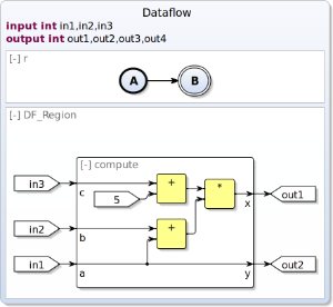
SCChart with Dataflow
SCG
Overview
Content Tools