The KGraph is the basic data structure used by the KIELER Infrastructure for Meta-Layout the Eclipse Layout Kernel (ELK) to describe and work with graphs. While developing layout algorithms, it is often necessary to assemble very specific graphs to see what the algorithm does with them. This is what the KGraph Text language was designed for: to be a simple language to assemble KGraphs for testing purposes.
This short tutorial will first introduce you to the KGraph and then walk you through writing your first KGT file. Grab a cup of tea and a few biscuits and work your way through it.
| Info | ||
|---|---|---|
| ||
Before starting the tutorial, make sure that you have either an Eclipse installation with the KIELER KGraph Editing and Visualization feature installed from our update site or our Standalone KGraph Editor. |
...
, slip into something more comfortable and get ready!
Preliminaries
There's a few things to do before we dive into the tutorial itself. For example, to do Eclipse programming, you will have to get your hands on an Eclipse installation first. Read through the following sections to get ready for the tutorial tasks.
Required Software
| Excerpt Include | ||||||
|---|---|---|---|---|---|---|
|
Finding Documentation
| Excerpt Include | ||||||
|---|---|---|---|---|---|---|
|
The KGraph
Take a look at the meta model on the KGraph Meta Model page. As you can see there, graphs consist of nodes and directed edges that connect the nodes. Nodes can declare special connection points called ports that edges can, but don't have to connect to. Nodes, ports, and edges can have labels that describe them. Since we don't want to pass lists of nodes around, each graph has a top-level node that contains the other nodes. This kind of parent-child relationship also enables us to describe nested graphs: graphs where nodes can contain further nodes themselves. So far, this is not all that surprising.
Our main goal with the KGraph is to have a data structure for layout algorithms. To compute a layout, we need to be able to specify the size and coordinates of each graph element. This is where the KLayoutData Meta Model comes into play. Each graph element can have arbitrarily many KGraphData elements attached to it. The KLayoutData meta model describes a number of such types that go with different graph elements:
| Graph Element | KGraphData Type |
|---|---|
KNode | KShapeLayout |
KPort | KShapeLayout |
KLabel | KShapeLayout |
KEdge | KEdgeLayout |
A shape has a size and width as well as coordinates and, possibly, insets. An edge has a starting point, an end point, and a list of bend points. Note that different coordinates have different frames of reference, as shown in the diagram below the KLayoutData meta model.
Layout algorithms will usually provide different options to configure them to your needs. To this end, each KGraphData class has a list of properties associated with it. Layout algorithms will go and evaluate properties as they compute layouts.
KGraph Text
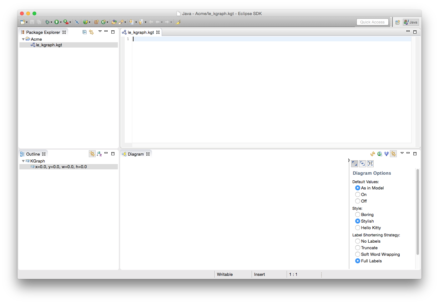
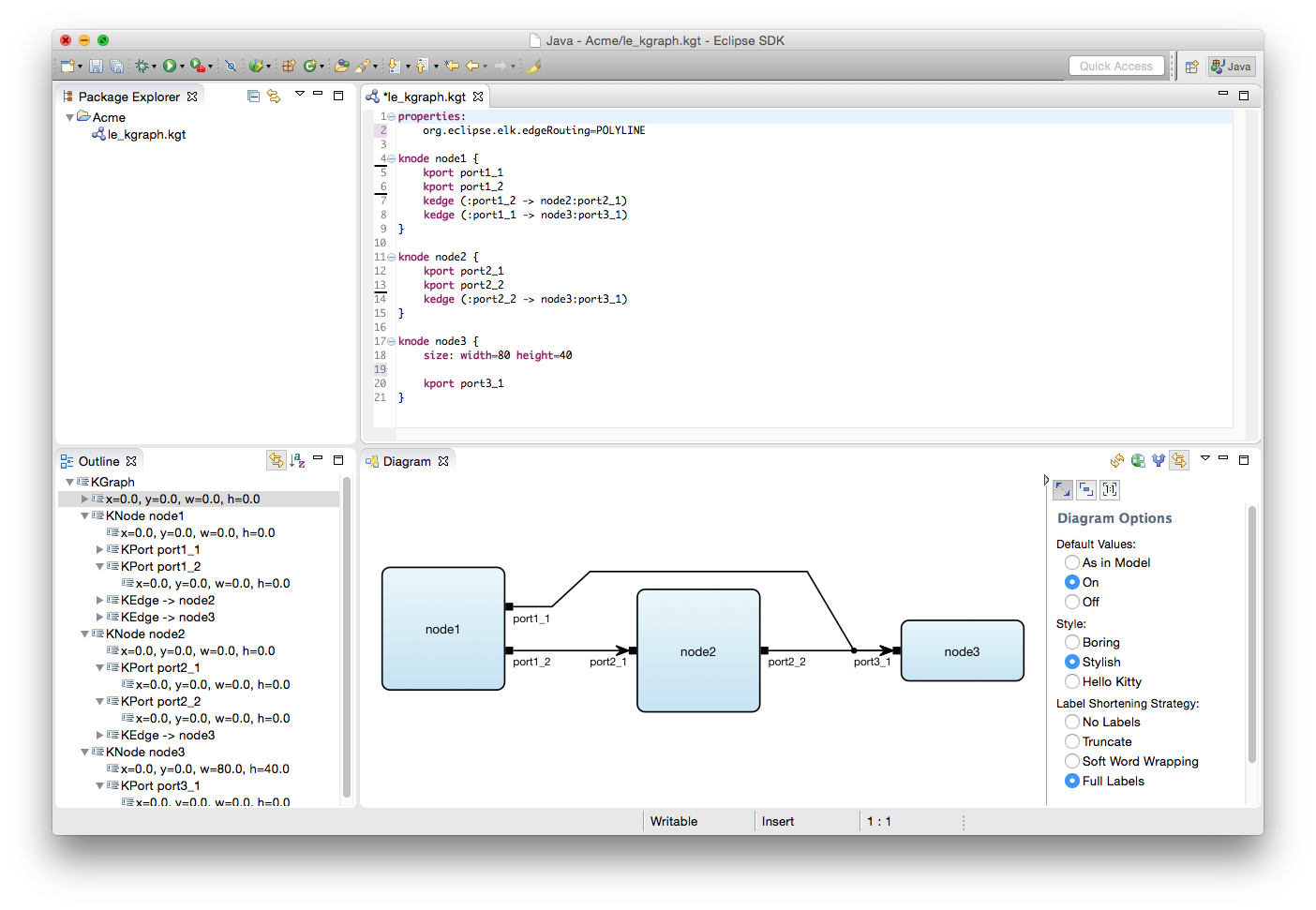
- When we cobble together our KGraph, it would be nice to see if what we type in makes any sense. As it turns out, we have actually built an Eclipse view that shows the graph as you type it in, but you will have to open that view first. From the Window menu, select Show View - Other.... In the dialog, select Diagram from the KIELER Lightweight Diagrams category. Your Eclipse window should look something like this:
- Create an empty project in your Eclipse workspace. Right-click the project and select New -> Other... In the dialog that pops up, select Empty KGraph from the KGraph category. Give the new file a proper name and click Finish to create it. Open the new file. Eclipse will ask you if you want to add the Xtext nature to your project. Click Yes. Don't worry about it.
- The KGraph editor should open , as should a KLighD viewand the Diagram view should update itself. Both should be empty, but the Diagram view should now show a handy sidebar that you can use to influence how your graph will be displayed. If the KGraph editor does not open, open the file yourself by double-clicking it in the Project Explorer.
Start by adding a few nodesfirst node. Enter the following text into the editor:
Code Block title Three nodeslinenumbers true knode node1 { size: width=100 height=100 }The KLighD view should update itself and show a rectangle that represents the node. Add two other , but you won't know since your node has no size yet and KLighD doesn't know how to draw it. Yep, that's not quite as helpful as you would have hoped. But alas, help is on its way!
- In the sidebar of the KLighD view, you can enable default values. Do so. (You can also enable stylish styling, which will improve the styling of the drawing style used to style nodes.)
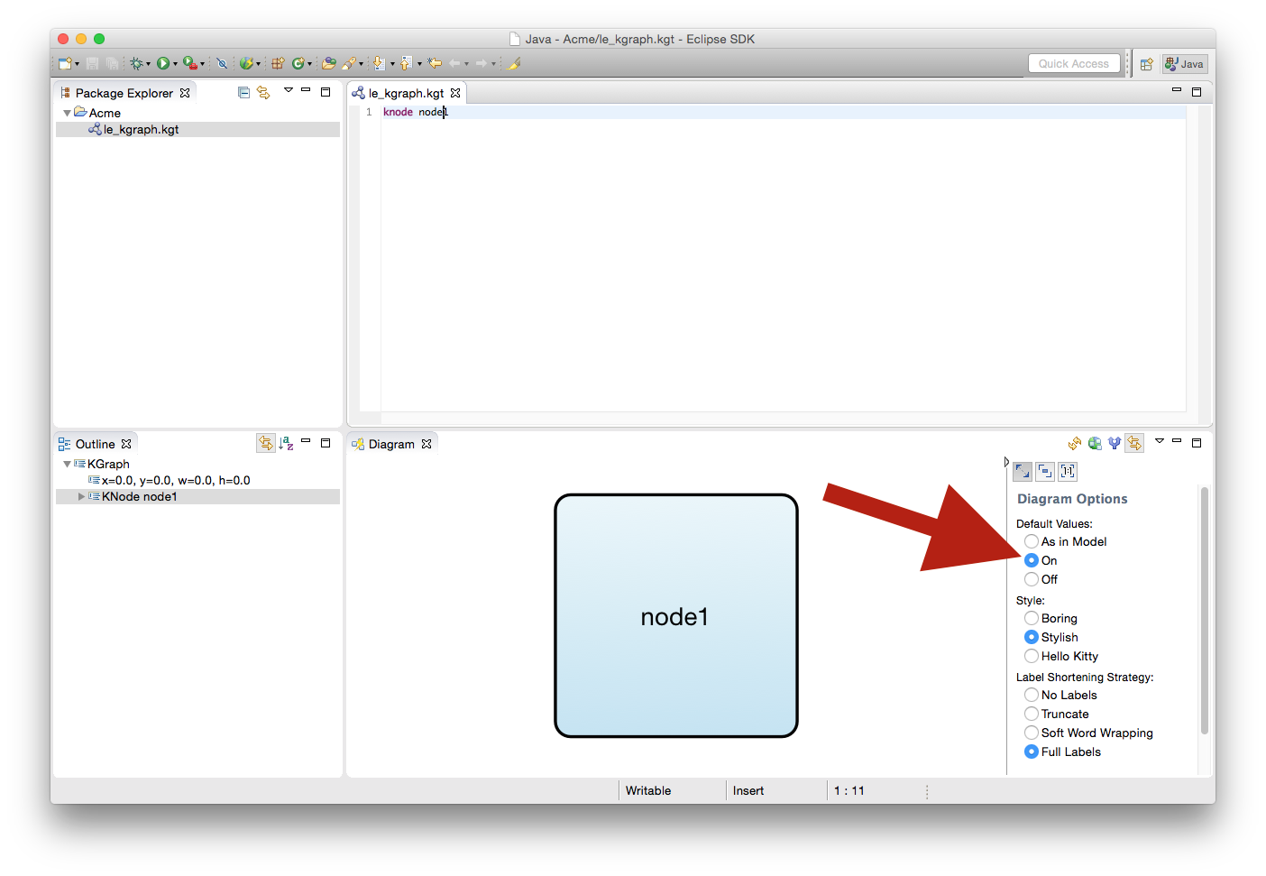
Your node now has a default label, a default size, and a default way to render it (a simple or a stylish rectangle). Add two further nodes,
node2andnode3, to the graph.Let's add connection points to the nodes. Add two ports tonode1by adding the following text under the size specification of the node:Code Block Nodes with ports linenumbers true kport port1_1 { size: width=10 height=10 } kport port1_2 knode node2 knode node3
Uniform sizes are boring, so let's give more individuality to
node3:Code Block linenumbers true knode node3 { size: width=1080 height=1040 }
One of the nodes in the KLighD view should now have black ports in the top left corner. This is of course not where we want the ports to end up, so we will have to tell the layout algorithm to place them wherever it's most convenient. The corresponding layout option is called port constraints. Add the following two lines under the size specification of
node1to set the proper constraints on it:Code Block title Port constraints linenumbers true properties: de.cau.cs.kieler.portConstraints=FREE
The KLighD view should be updated again and place all ports on the left side of their node. Add two ports,Info title Hint The KGT editor has auto completion that you can trigger by pressing Ctrl+Space. The list that pops up shows you everything that can be added at the current cursor position. This is especially handy when it comes to property IDs and possible property values.
Let's add connection points to the nodes. Add two ports to
node1:Code Block linenumbers true knode node1 { kport port1_1 kport port1_2 }Two black rectangles should now appear at
node1. If we had turned off default values, the ports would not have a proper size and would miss their labels.- Add a port
port2_1andport2_2, tonode2. Also, add tonode2and a portport3_1tonode3. It's now time to connect the nodes. Add two edges to the graph that originate at
node1by adding the following lines under the port definitions ofnode1:Code Block title Edgeslinenumbers true kedge (:port1_2 -> node2:port2_1) kedge (:port1_1 -> node3:port3_1)
Edges can start and end at a node or at a port. The source node does not need to be explicitly specified since it is clear from the context (the edges are defined in the body of the source node, after all). Thus, if an edge connects directly to the source node (that is, not through a port), the part before the arrow (
->) will be empty. The target needs the node to be specified, with an optional target port. Add another edge that starts atport2_2and ends atport3_1. By now, the KLighD view should show something like this :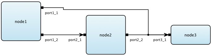
One of the problems here is that it is not immediately clear from the drawing which rectangle belongs to which node. This can easily be remedied by adding labels. Start by adding a label to the first node:
Code Block title Labels linenumbers true klabel "Node 1"In the same way, add labels to the other nodes. You will notice that the placement of the labels is not very good. Add the following line to the
propertiessection of each node:Code Block title Label placement linenumbers true de.cau.cs.kieler.nodeLabelPlacement="INSIDE H_LEFT V_TOP"This will place the labels at the top left corner inside each node. Of course, there are other possible placements you can experiment with. Note that while the value of the port constraints option above could be simply written as
FREE, the value of this option needs to be put in quotation marks. This is because this option's value is actually a set of values.Tip title Try this Labels can also be added to ports and are then properly placed by the layout algorithm as well...
(with stylish styling enabled, of course):
Let's add a final touch to the graph. Currently, the edges are routed as polylines with slanted edge segmentsorthogonally. If we want to change that, we need to tell the layout algorithm to use another edge routing algorithm. This can be done by attaching a layout option to our graph. Add a new
propertiessection to the beginning of the file:Code Block title Edge Routinglinenumbers true properties: deorg.caueclipse.cselk.kieler.edgeRouting=ORTHOGONALPOLYLINEYour result could look something like this:
...
Tip title Properties Properties can be attached to just about anything in a KGraph: the graph itself, nodes, ports, labels, ...
Okay, how about a final final touch. The node labels are currently centered inside their nodes. You can change that by adding the following property to, say,
node1:Code Block linenumbers true org.eclipse.elk.nodeLabels.placement="OUTSIDE V_BOTTOM H_CENTER"This will center its label below the node.
Right, that concludes our little tutorial. If you want to go further, read more on the KGT syntax and look at a bigger example. Also, solve the following assignment.
| Panel | ||
|---|---|---|
| ||
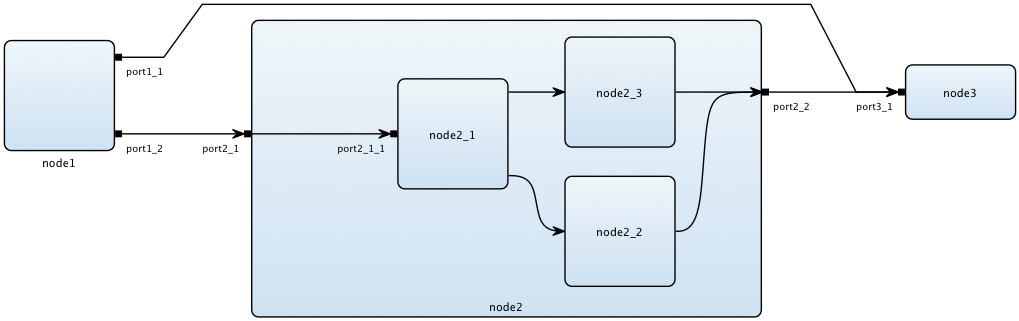
Graphs can also be nested. Child nodes are added to a parent node just like you added ports to parent nodes. Try to extend the graph above such that it looks like this:
Note that the edges inside |