...
The imported projects contain a meta model for Turing machines. (You may notice that this tutorial thus also slips in a perfect opportunity to brush up on your knowledge of Turing machines. Consider it a public service and thank us later.) It does not model the tape or the head, only its states and transitions. It is these Turing machines that we will develop a visualization for over the course of this tutorial.
Creating a Visualization
Now that we have the model of what we want to visualize, it's time to program the actual visualization. But first, let's take a minute to think about what we need to do here. Take a look at the following diagram:
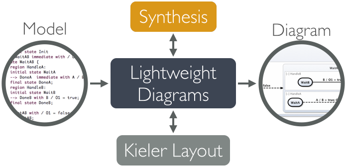
In our visualization, what we have is an instance of a Turing machine model, and what we want to end up with is a proper diagram that visualizes it. Of course, Lightweight Diagrams has not the slightest clue about what we want our diagrams to look like. That is where the synthesis, highlightes above, comes into play. The synthesis is what transforms an instance of our source model into a KGraph that Lightweight Diagrams knows how to render. (Along the way, KIELER Layout is invoked by KLighD to compute positions for all diagram elements.)
Right, let's dive right in and develop our synthesis.
Adding a Visualization Project
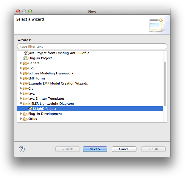
- Right-click in the Package Explorer and select New -> Other. From the list, select KIELER Lightweight Diagrams -> KLighD Project.
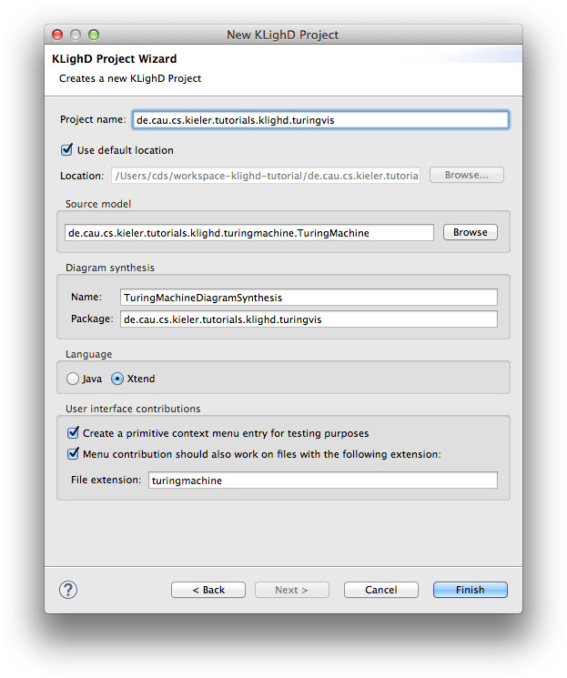
- Give your new project a proper name and select the base element of the model you want to visualize. Here's what you should enter here before clicking Finish: