KIELER Lightweight Diagrams (KLighD) allows you to develop visualizations for data structures quite easily. In this tutorial, we will install Eclipse and all the necessary components to develop KLighD visualizations before moving on to actually develop a visualization of a state machine.:
| Warning |
|---|
TODO: Add a screenshot of what the outcome of this tutorial will be. |
Preliminaries
There's a few things to do before we dive into the tutorial itself. For example, to do Eclipse programming, you will have to get your hands on an Eclipse installation first. Read through the following sections to get ready for the tutorial tasks.
...
- Download the zip file with all our prepared tutorial plugins from our Stash. Unzip the file.
- Open the context menu within the Package-Explorer (on the very left, right-click the empty space).
- Select Import. Then chose General > Existing Projects into Workspace.
- Browse to the location where you unzipped the downloaded plug-ins. Check the checkbox check box in front of all the
de.cau.cs.kieler.tutorials.klighd.*projects and press Finish.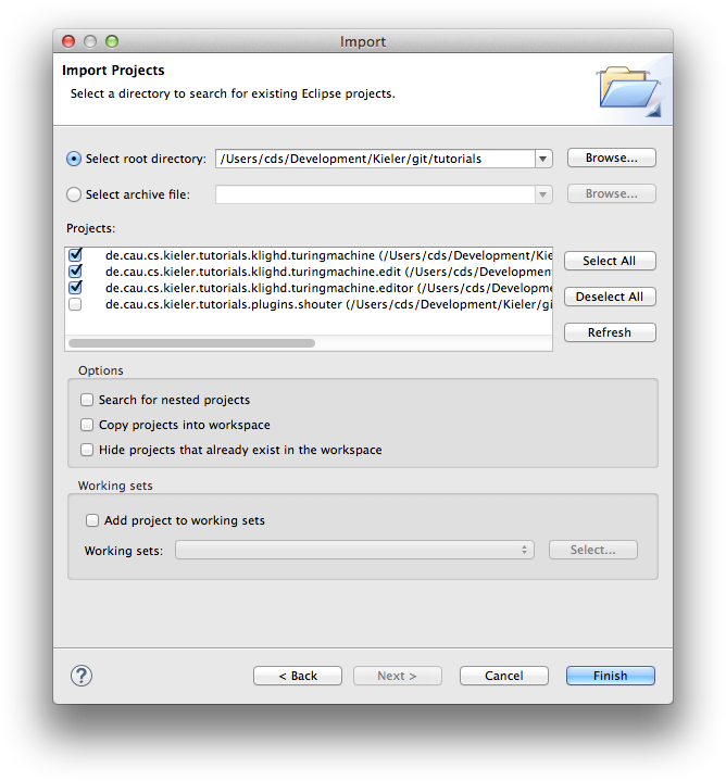
The imported projects contain a meta model for Turing machines. (You may notice that this tutorial thus also slips in a perfect opportunity to brush up on your knowledge of Turing machines. Consider it a public service and thank us later.) It does not model the tape or the head, only its states and transitions. It is these Turing machines that we will develop a visualization for over the course of this tutorial.
| Tip | ||
|---|---|---|
| ||
Should your projects be marked with a big red exclamation mark, there might be build path problems. To fix them, complete these steps with all such projects:
If that wasn't the source of the problem, ask your advisor. |
Creating a Visualization
Now that we have the model of what we want to visualize, it's time to program the actual visualization. But first, let's take a minute to think about what we need to do here. Take a look at the following diagram:
...
In our visualization, what we have is an instance of a Turing machine model, and what we want to end up with is a proper diagram that visualizes it. Of course, Lightweight Diagrams has not the slightest clue about what we want our diagrams to look like. That is where the synthesis, highlightes highlighted above, comes into play. The synthesis is what transforms an instance of our source model into a KGraph that Lightweight Diagrams knows how to render. (Along the way, KIELER Layout is invoked by KLighD to compute positions for all diagram elements.) However, the KGraph itself does not suffice to render the diagram: it only specifies its structure, but not its appearance. To specify the latter, we also need to augment our KGraph by KRendering information. See its documentation to learn more about what it can do.
...
We will now start filling in the synthesis skeleton, so open the TuringMachineDiagramSynthesis class:
| Code Block | ||||
|---|---|---|---|---|
| ||||
/* Package and import statements... */

class TuringMachineDiagramSynthesis extends AbstractDiagramSynthesis<TuringMachine> {

    @Inject extension KNodeExtensions
    @Inject extension KEdgeExtensions
    @Inject extension KPortExtensions
    @Inject extension KLabelExtensions
    @Inject extension KRenderingExtensions
    @Inject extension KContainerRenderingExtensions
    @Inject extension KPolylineExtensions
    @Inject extension KColorExtensions
    extension KRenderingFactory = KRenderingFactory.eINSTANCE


    override KNode transform(TuringMachine model) {
        val root = model.createNode().associateWith(model);

        // Your dsl element <-> diagram figure mapping goes here!!

        return root;
    }

} |
...
Add a new method to your synthesis that transforms a
Stateinto a correspondingKNode:Code Block language javascala linenumbers true private def KNode transform(State state) { val stateNode = state.createNode().associateWith(state); return stateNode; }While this method does indeed create a node for the state passed to it, KLighD wouldn't know how to render it yet. Let's draw the node as a rounded rectangle by adding the following line before the
returnstatement:Code Block language java linenumbers true stateNode.addRoundedRectangle(4, 4, 2);
The only thing missing now is a label with the state's name:
Code Block language java linenumbers true stateNode.addInsideCenteredNodeLabel(state.name, KlighdConstants.DEFAULT_FONT_SIZE, KlighdConstants.DEFAULT_FONT_NAME); stateNode.addLayoutParam( LayoutOptionsCoreOptions.NODE_SIZE_CONSTRAINTCONSTRAINTS, EnumSet.of(SizeConstraint.MINIMUM_SIZE, SizeConstraint.NODE_LABELS));Now that we know how to transform states, we have to call our new method from the main transformation method. Replace the comment in its body with the following line of code:
Code Block language scala linenumbers true model.states.forEach[ s | root.children += transform(s) ]
Let's see if our visualization works. Start your program (if you don't know how to do that, check out our Eclipse Plug-ins and Extension Points tutorial) and follow these steps:
- Right-click the Package Explorer and select New -> Project.
- In the dialogdialogue, select General -> Project and click Next.
- Give the project a meaningful name (Foo is a classic) and click Finish.
- Right-click your new project in the Package Explorer and select New -> Other.
- In the dialogdialogue, select Example EMF Model Creation Wizards -> Turingmachine Model and click Next.
- Give your Turing machine file a meaningful name (Bar.turingmachine is a classic) and click next.
- As the Model Object, select Turing Machine, which is the root element of our model. Click Finish.
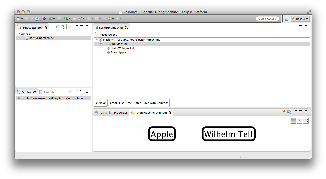
- In the editor that opens, expand the first row. Make sure the Properties view is open by right-clicking in the editor and selecting Show Properties View.
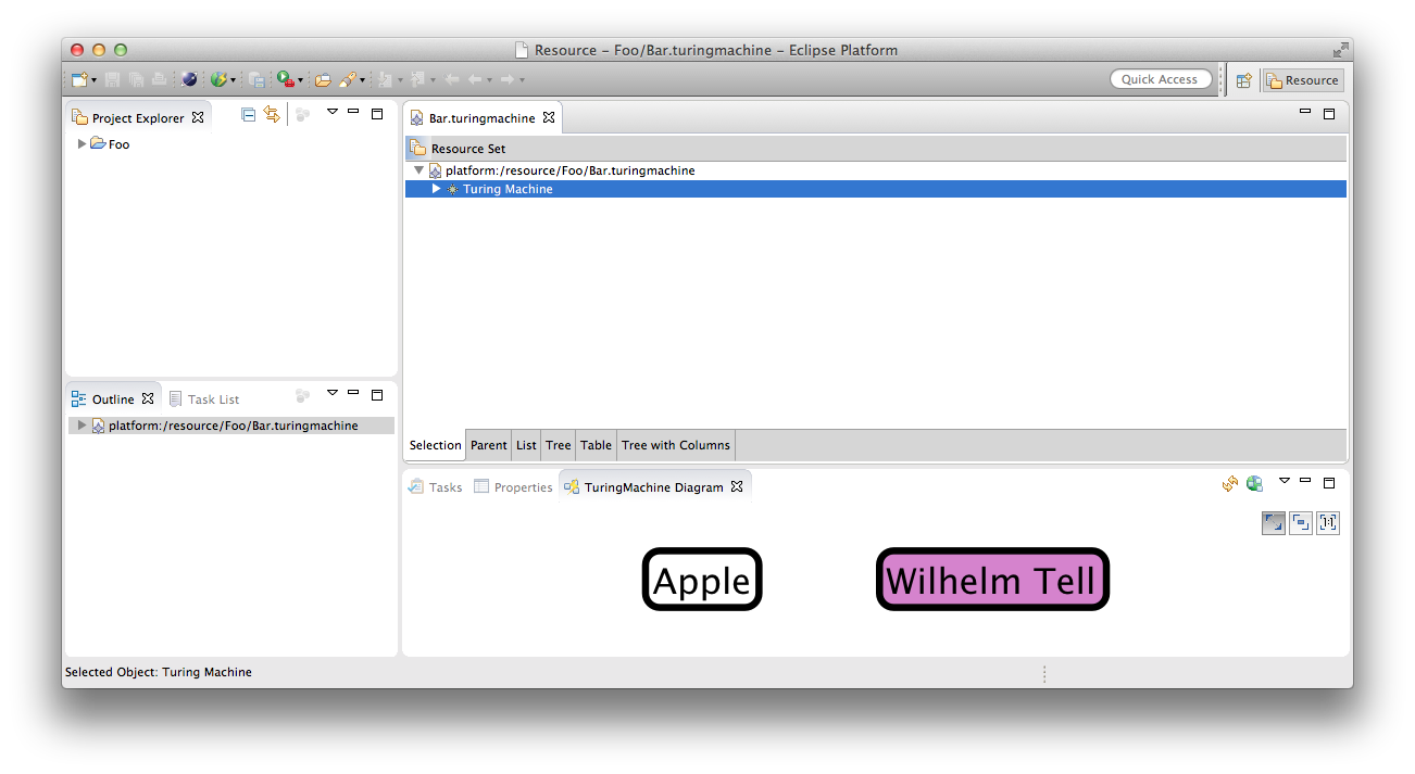
- Right-click Turing Machine and select New Child -> State. Give the state a name through the properties view, such as Wilhelm Tell. Also mark it as the initial state of the Turing machine.
- Add another, non-initial state named Apple.
- Save the file.
To test your visualization, you can right-click either the file in the Package Explorer or the Turing Machine row in the editor and select Open TuringMachine diagram. A KLighD view should open and display something like this:
That's quite nice already, but we have no way to determine which of these states is the default. Let's add a hideously ugly background colour to initial states by changing the line that adds a rounded rectangle:
| Code Block | ||||
|---|---|---|---|---|
| ||||
stateNode.addRoundedRectangle(4, 4, 2) => [ rect |
    if (state.initial) {
        rect.setBackgroundColor(210, 130, 210);
    }
]; |
The result should look something like this (I told you it was going to be hideous):
Visualizing Transitions
Now that we have our states, it's time to visualize transitions as well. It would be nice to just transform transitions leaving a given state while we're transforming that state. Let's do that:
Add the following code right before the
returnstatement in the state transformation method:Code Block language scala linenumbers true stateNode.outgoingEdges.addAll(state.outgoingTransitions.map[ t | transform(t) ])Of course, we will have to add a
transformmethod for transitions now:Code Block language scala linenumbers true private def KEdge transform(Transition trans) { val transEdge = trans.createEdge().associateWith(trans) return transEdge; }Again, we need to tell KLighD how to render the label:
Code Block language java linenumbers true transEdge.addPolyline(2).addHeadArrowDecorator();And the edge also needs a label that describes the transition:
Code Block language scala linenumbers true // Add a label to the edge val label = KGraphUtil.createInitializedLabel(transEdge); val labelText = trans.trigger + " / " + trans.action + " " + trans.direction + " " + trans.newChar; label.configureCenterEdgeLabel(labelText, KlighdConstants.DEFAULT_FONT_SIZE, KlighdConstants.DEFAULT_FONT_NAME);What is missing now is to set the edge target to the node that represents the target state. There's a problem here, though: we don't even know if the target state already had a node created for it. Thus, we need to make sure it has:
Code Block language java linenumbers true transEdge.target = transform(trans.targetState);This, however, results in a different problem: if the target state already had a node created for it, we now create another node. What we would need the state transformation method to do would be to first check if a node has already been created for a given state, and, if so, return that instead of creating a new one. It turns out that Xtend already supports this pattern. Change the method's declaration and its first line to the following:
Code Block language scala linenumbers true private def create stateNode : state.createNode() transform(State state) { stateNode.associateWith(state);Also, remove the return statement. Xtend now checks if we already created a node for the given state and, if not, execute the code in the method.
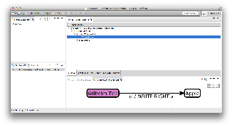
Start your program again, open your Turing machine file
...
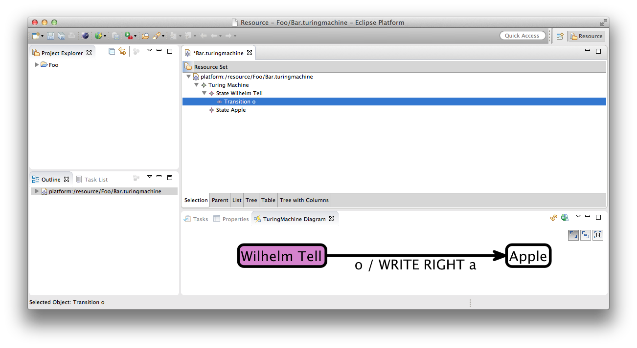
and add an outgoing transition to your Wilhelm Tell state. Change the properties 'New Char' and 'Trigger' to arbirtary characters (but not 0, since that translates to the ASCII char null and will kill your Label). Set the Apple state as the transition's target state. Save the model and fire up a KLighD view. It should look something like this:
Going Further
This concludes our little KLighD tutorial, but of course there's a lot you haven't seen yet. To go further, take a look at the KLighD pages in our KIELER Confluence space and the examples described there. Also, try solving the assignment below, if you like.
| Panel | ||
|---|---|---|
| ||
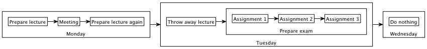
In text files, lists can be written like this:
Create a new project that provides a menu item that fires up a visualization for this kind of list format. The visualization should look something like this:
When parsing the string, you can simply assume that each level of the list gets indented by exactly two spaces, and that the text of each list item starts after an asterisk followed by a space. No need to build fancy error checking into your solution. |