Page History
| Panel | ||
|---|---|---|
| ||
Responsible: |
The KGraph Text (KGT) project provides a textual syntax and editor for specifying KGraphs. While editing the KGraph in the textual editor, we provide a visualization of the graph in a KLighD view. This project was started with two use cases in mind:
...
| Table of Contents |
|---|
Quick Start Tutorial
This short tutorial will walk you through writing your first KGT file. Grab a cup of tea and a few biscuits and work your way through it.
| Info | ||
|---|---|---|
| ||
Before starting the tutorial, make sure that you have an Eclipse installation with the KIELER KGraph Editing and Visualization feature installed. |
...
Start by adding a few nodes. Enter the following text into the editor:
| Code Block | ||||
|---|---|---|---|---|
| ||||
knode node1 {
    size: width=100 height=100
} |
The KLighD view should update itself and show a rectangle that represents the node. Add two other nodes, node2 and node3, to the graph.
Let's add connection points to the nodes. Add two ports to node1 by adding the following text under the size specification of the node:
| Code Block | ||||
|---|---|---|---|---|
| ||||
kport port1_1 {
    size: width=10 height=10
}

kport port1_2 {
    size: width=10 height=10
}
|
One of the nodes in the KLighD view should now have black ports in the top left corner. This is of course not where we want the ports to end up, so we will have to tell the layout algorithm to place them wherever it's most convenient. The corresponding layout option is called port constraints. Add the following two lines under the size specification of node1 to set the proper constraints on it:
| Code Block | ||||
|---|---|---|---|---|
| ||||
    properties:
de.cau.cs.kieler.portConstraints=FREE |
| Info | ||
|---|---|---|
| ||
The KGT editor has auto completion that you can trigger by pressing Ctrl+Space. The list that pops up shows you everything that can be added at the current cursor position. This is especially handy when it comes to property IDs and possible property values. |
...
It's now time to connect the nodes. Add two edges to the graph that originate at node1 by adding the following lines under the port definitions of node1:
| Code Block | ||||
|---|---|---|---|---|
| ||||
kedge (:port1_2 -> node2:port2_1)
kedge (:port1_1 -> node3:port3_1) |
Edges can start and end at a node or at a port. The source node does not need to be explicitly specified since it is clear from the context (the edges are defined in the body of the source node, after all). The target needs the node to be specified, with an optional target port. Add another edge that starts at port2_2 and ends at port3_1. By now, the KLighD view should show something like this: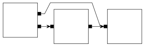
...
One of the problems here is that it is not immediately clear from the drawing which rectangle belongs to which node. This can easily be remedied by adding labels. Start by adding a label to the first node:
| Code Block | ||||
|---|---|---|---|---|
| ||||
klabel "Node 1" |
In the same way, add labels to the other nodes. You will notice that the placement of the labels is not very good. Add the following line to the properties section of each node:
| Code Block | ||||
|---|---|---|---|---|
| ||||
de.cau.cs.kieler.nodeLabelPlacement="INSIDE H_LEFT V_TOP" |
This will place the labels at the top left corner inside each node. Of course, there are other possible placements you can experiment with. Note that while the value of the port constraints option above could be simply written as FREE, the value of this option needs to be put in quotation marks. This is because this option's value is actually a set of values.
| Tip | ||
|---|---|---|
| ||
Labels can also be added to ports and are then properly placed by the layout algorithm as well... |
...
Let's add a final touch to the graph. Currently, the edges are routed as polylines with slanted edge segments. If we want to change that, we need to tell the layout algorithm to use another edge routing algorithm. Add a new properties section to the beginning of the file:
| Code Block | ||||
|---|---|---|---|---|
| ||||
properties:
de.cau.cs.kieler.edgeRouting=ORTHOGONAL |
Your result could look something like this:
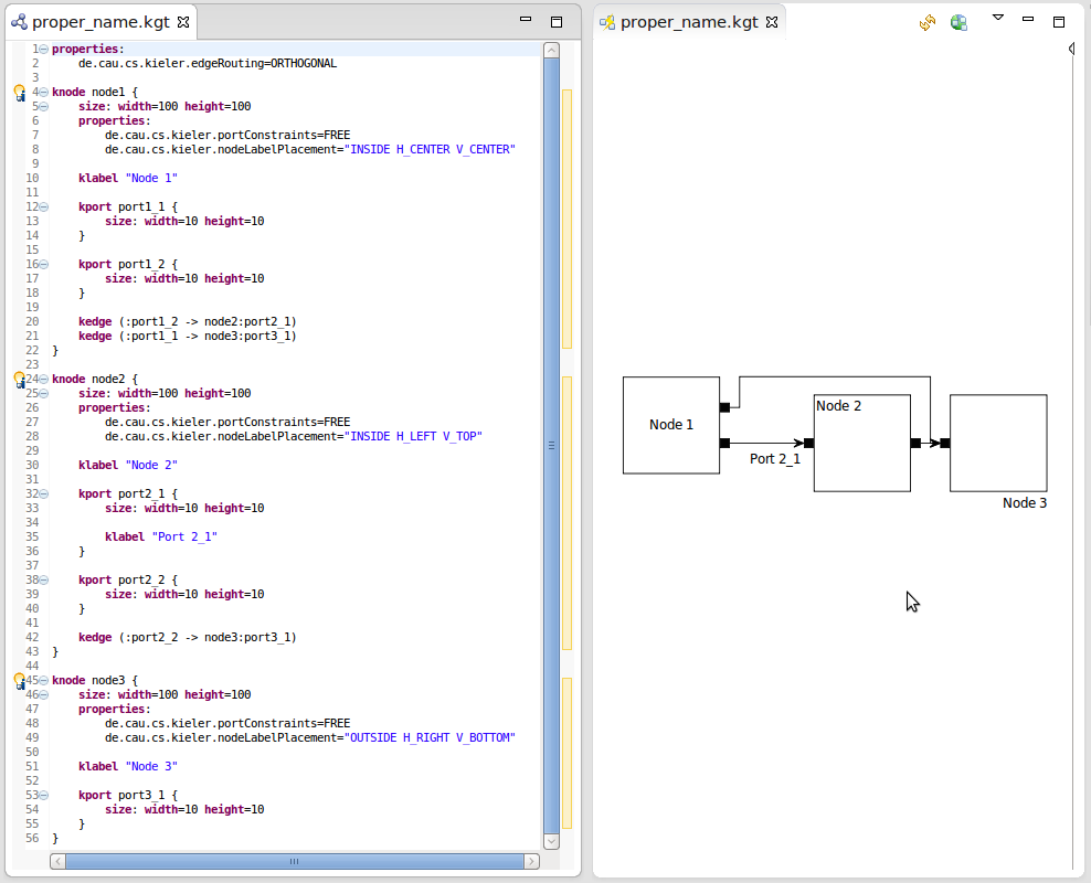
So much for a first glance at how KGT editing works. The rest of this page is devoted to a more detailed explanation of the syntax of the formatTo quickly get you up to speed on how to write basic KGT files, we have a full-blown tutorial available for you learning pleasure. Once you've completed that, the rest of this page will provide a more comprehensive description of the KGT syntax.
The KGraph Text Format
In this section, we will take a closer look at the KGT syntax. We will start with the basic syntax. We will then take a look at the different kinds of objects available in KGT and at specifying parameters and properties of these objects.
...
| Code Block | ||||
|---|---|---|---|---|
| ||||
properties:
    de.cau.cs.kieler.algorithm="de.cau.cs.kieler.klay.tree"

knode n1 {
    size: width=50 height=50

    kedge (-> n2)
    kedge (-> n3)
}
knode n2 {
    size: width=50 height=50
}
knode n3 {
    size: width=50 height=50
} |
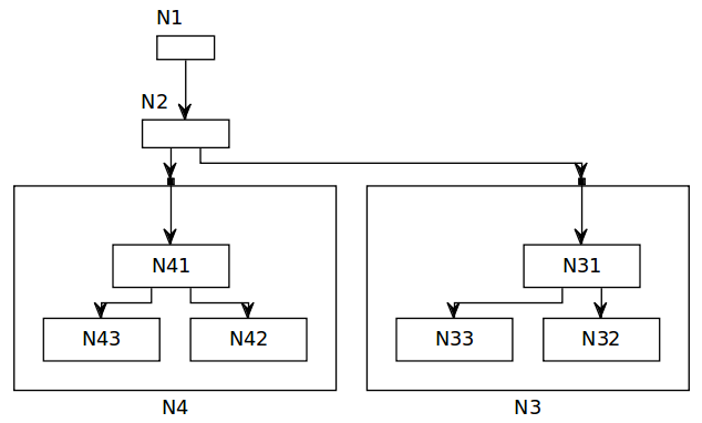
A More Complex Example
We finish with a more complex example that highlights some of the features of the KIELER graph layout technology and how to use it through the KGT format.
| Section | |||||||||||
|---|---|---|---|---|---|---|---|---|---|---|---|
|
Overview
Content Tools