The KRendering Notation Model

See also KGraph and KLayoutData.

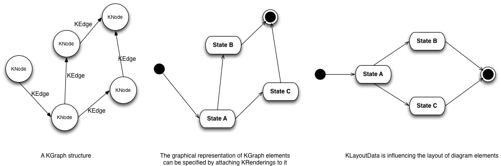
The KRendering data structure is used to specify the visual representation of a KGraph structure. Therefor an individual KRendering gets attached to each KGraph element defining its appearance. A full KRendering visualization utilizes three meta models:

•  The KGraph model defines the structure.
•  The KLayoutData model defines the graph layout.
•  The KRendering model defines the rendering of KGraph elements

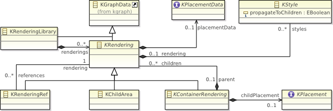
The KRendering class is the base class of all renderings. More complex renderings can be build-up of multiple simple drawings using the KContainerRendering class which is the base class of all renderings with children. The KChildArea class can be used to place a KNode at a specific position inside a rendering. Once you have created a figure, KRendering offers the possibility to store it in a KRenderingLibrary. A stored rendering can be reused by referencing it with a KRenderingRef.

The following figure shows basic container renderings.

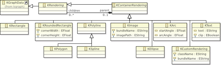
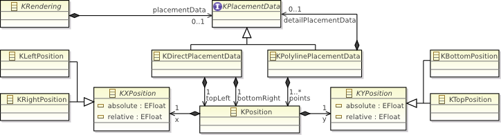
Children of KContainerRenderings are placed inside, depending on the KPlacement of the container. Currently KRendering offers KStackPlacement for placing renderings in one column and KGridPlacement for placing renderings on a grid. KDirectPlacement is the default placement of all renderings. A children's placement can be refined by attaching KPlacementData to it. For example by using KDirectPlacementData you can specify the bounding box of a KRendering. The coordinates are relativ to left/right and top/bottom of the parent and have an absolute and relative part.

Rendering details e.g. LineWidth, ForegroundColor, Foreground visibility are specified by lists of KStyle objects. The convention is that early styles in the list overwrite later ones. By setting the attribute propagateToChildren you can apply the style to all children of the rendering.

Working with the KLighD editor

Installing the required plugins

Before we can start with creating diagrams, we have to install the necessary plugins into our Eclipse IDE. The easiest way getting the latest release is downloading it from the KIELER git repository. 

 See here a detailed documentation on this topic:

http://www.rtsys.informatik.uni-kiel.de/confluence/display/KIELER/Using+Git

Testing the KlighD installation

If you have followed the steps on the linked page above, you should have a working KIELER environment including KLighD. To make sure that this is true, you can follow these steps to create a simple KLighD visualization.

1. Create an empty Project by selecting: 
1. File->New->Project 
2. choose General->Project and click next
3. type in a name for the new project like: de.klighd.test
2. Create a new KGraph file by right clicking on the new project in the Eclipse Project Explorer and then
1. New->File
2. type in a name for the file like test.kgraph
3. be sure you have included the file extension '.kgraph' before clicking on finish as Eclipse is using this extension to open the correct Editor for this file.
3. Finally double click to open this file and copy the following lines of code into the editor that pops up.
    

KNode { 
	children:
	KNode {
		data:
		KShapeLayout
		{
			width 100
			height 100
		}
	}	
} 

We will discuss in the later sections what this code means.

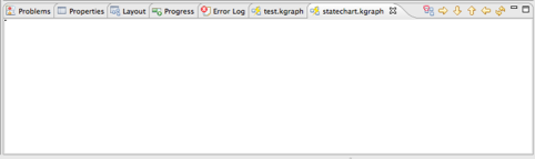
For the moment you should be satisfied by seeing a new view popping up that looks like this:

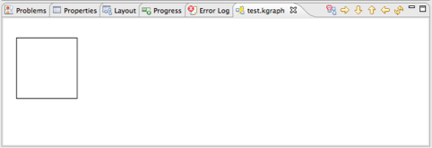
If you don‘t see it, try selecting: window->open view->Light Diagram.

KLighD Basics

In this section we will look at basic concepts behind a KLighD visualization to understand how the involved data structures specify a graphical diagram.

First of all there is the KGraph data structure which serves as specification for the structure of the diagram. Like the name implies, this is done by defining a graph structure using KNodes and KEdges.

A KNode represents one single diagram figure and can be connected width KEdges.

However, these objects doesn't have graphical representations before you attach additional data to them. There are two sorts of Information that you can attach to your KGraph data structure.

1.KRendering data

You can use KRendering data  to specify how graph elements were drawn. Therefor, the KRendering meta model provides basic graphical figures like rectangles, text elements, lines and properties like text size or background color.

2.KLayoutData

By attaching KLayoutData to KGraph objects, you can specify how these elements are handled by during the layout phase. This means, you can choose a layout algorithm and define properties for it.

Using the textual KGraph Editor

In this chapter we will use the textual KGraph Editor to create a prototype for a simple state diagram.  

Prerequisites

1. Follow the steps 1 and 2 of the section ,Testing the Klighd installation‘ to create a new file with the name ,statechart.kgraph‘ and open the editor by double clicking on it.
2. Every klighd visualization need a root node. Think of it as the canvas where you placing Objects on. To create a node just type in the following lines: 

KNode { 

}

Notice: You can use the eclipse content assist (press ctrl + space) to get hints on what statement the syntax expects from you.

A Simple Rendering

1. Now attach a new child node to it by adding the following lines between the curly brackets of the root node:

children:
KNode{

}

 This node should later represent a simple state.

 2. To archive this, we must attach KRenderings to it. Do this by adding the following lines between the curly brackets of the node.

data:
RoundedRectangle 30 30 {
			
}

As you can probably guess, these lines should specify the graphical representation of this node to an rounded rectangle with corner width/height set to 30.

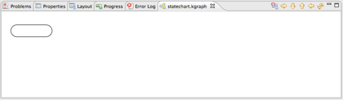
When you open the Light Diagram view (if it isn’t already) Window -> Show View -> Light Diagram the result of this code is probably not what you would have expected.

As you can see, the view shows only a little dot.  The reason for this is, that we don‘t have specified the size of the graphical element. We do this by adding a KShapeLayout to the KNode data. Please change the code to match the following lines:

KNode { 
	children:
	KNode{
		data:
		KShapeLayout{
			width 100 height 30
		},
		RoundedRectangle 30 30 {
	
		}		
	}	
}

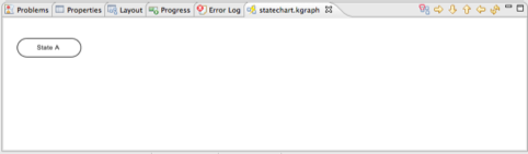
Here we added a KShapeLayout that is setting the width and height of the graphical Element. The result should look like this.

3. The next step is to add a label to denote the name of the state. Because the Object of the rounded rectangle is of type container rendering, we can add child renderings to it. So we can simply add a KText as child element to the rectangle.

RoundedRectangle 30 30 {
	children:
	Text "State A" {

	}
  }

As a result we have a  complete visualization of at least one simple state.

Connecting diagram elements.

This section explains how edges can be used to connect diagram elements. Before we can begin with this, we have to add a second graph element. You can copy the existing KNode. The children of KNodes are syntactically separated by a comma. 

The code should now look like this:

KNode { 
	children:
	KNode{
		data:
		KShapeLayout{
			width 100 height 30
		},
		RoundedRectangle 30 30 {
			children:
			Text "State A" {
				
			}
		}		
	},
	KNode{
		data:
		KShapeLayout{
			width 100 height 30
		},
		RoundedRectangle 30 30 {
			children:
			Text "State B" {
				
			}
		}		
	}	
}

1.To create an outgoing edge, simply write the following directly after the source KNode specification.

KNode{
	// ...
} --> "//@children.0" { 
	data :
	KEdgeLayout {
		sourcePoint KPoint x 0 y 0 
		targetPoint KPoint x 0 y 0 
	},
	Polyline {
		
	}
}

The ,-->‘ serves as prefacing operator for edges and is followed by a String addressing the target. In this case the first child of the root node which is our node representing State A.

It is important to attach an KEdgeLayout to the edge even if the source and target points can be set random numbers. The layout algorithm will change these values during the layout phase.

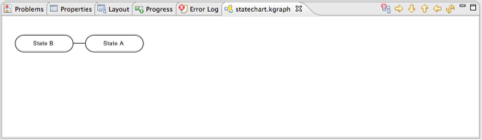
The light diagram view should now display something like this:

Using placement data to create complex renderings.

This section should explain how complex rendering can be build up of simple ones, using placement data. 

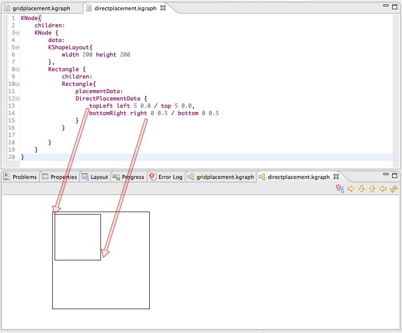
KDirectPlacement

Direct placement is the default placement data. With KDirectPlacmentData you can define the bounding box for the rendering. 

This must be done by specifying the coordinates of the top left and bottom right corner of the bounding box relative to the bounds of the parent rendering.

For both the horizontal and the vertical part of the coordinate, three values must be set:

The effects of the values chosen in 1. and 2. will be combined by addition.

The following example shows how this placement can be used to specify the position of child renderings.

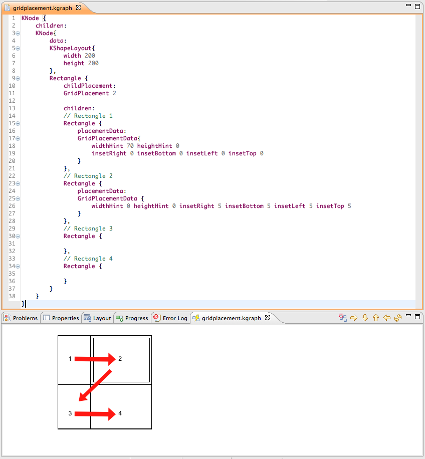
KGridPlacement

Grid placement is another possibility KLighD offers to arrange child renderings. As the name suggest, you can use it to place child rendering on a grid. You can later refine this placement by using KGridPlacementData.

The following picture shows an example where grid placement is used to arrange four rectangles on a grid with two columns.

As you can see, the rectangles where placed in syntactical order from left to right and top to bottom on the grid.

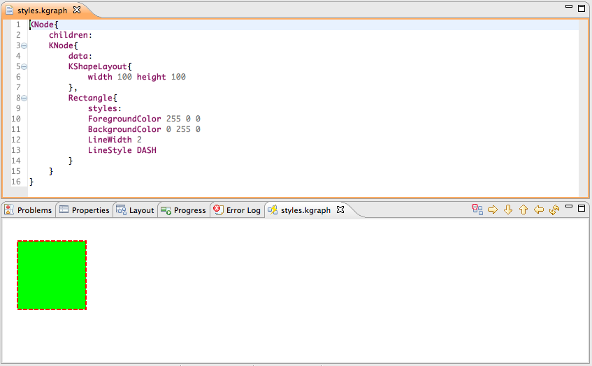
Using Styles

You can specify rendering details of KRenderings by adding styles to them.  Simply type in ,styles:‘ followed by a list of the desired styles. Use the content assist for a hint on which styles are available.

Here is an example: